In-class Exercise 3

Updated this exercise with kriging

1 About this Exercise

In this exercise we will learn how to create an isohyet map using R.

What is an isohyet map?

It is a map depicting contours of equal precipitation amounts recorded during a specific time period.

source

To prepare an isohyet map, we will need to do spatial interpolation. Spatial interpolation is the process of using points with known values to estimate values at other unknown points. For example, we only have weather stations at certain areas in Singapore. As weather stations do not cover the entire Singapore area, we would need to do spatial interpolation to estimate the rainfall at areas without recorded rainfall reading using the known rainfall readings at nearby weather stations. There are many interpolation methods. This type of interpolated surface is often called a geostatistical surface.

In this hands-on exercise, two widely used spatial interpolation methods called Inverse Distance Weighting (IDW) and kriging will be introduced.

2 Getting Started

2.1 Installing the Relevant Packages

For this exercise, other than tidyverse, we will be using the following packages:

• sf: allow us to data import and manipulate geospatial data

• terra: allow us to create grid (also known as raster) objects as the input and output of spatial interpolation.

• gstat: for spatial and spatio-temporal geostatistical modelling, prediction and simulation. In this in-class exercise, it will be used to perform spatial interpolation.

• tmap: allow us to visualise spatial data

• viridis: a colour library

• automap: for performing automatic variogram modelling and kriging interpolation.

pacman::p_load(sf,terra, gstat, tmap, viridis, tidyverse, automap)

2.2 Importing the Data

2.2.1 Rainfall Station Data

In the code chunk below, read_csv() of readr package is used to import RainfallStation.csv. We will call the imported data rfstations. From the output using str(), we noted that rfstations is in tibble data.frame format and it has three columns: Station, Latitude and Longitude.

rfstations <-read_csv("data/aspatial/RainfallStation.csv")
str(rfstations)

spc_tbl_ [63 × 3] (S3: spec_tbl_df/tbl_df/tbl/data.frame)
 $ Station  : chr [1:63] "Admiralty" "Admiralty (West)" "Ang Mo Kio" "Boon Lay (East)" ...
 $ Latitude : num [1:63] 1.44 1.46 1.38 1.33 1.33 ...
 $ Longitude: num [1:63] 104 104 104 104 104 ...
 - attr(*, "spec")=
  .. cols(
  ..   Station = col_character(),
  ..   Latitude = col_double(),
  ..   Longitude = col_double()
  .. )
 - attr(*, "problems")=<externalptr> 

2.2.2 Rainfall Records Data

In the code chunk below, read_csv() of readr package is used to import DAILYDATA_202402.csv. We will call the imported data rfdata. In addition to importing the data, we also use select() to retain column 1 and 5 of the imported data, then we use group_by() and summarise() to compute the total monthly rainfall from Daily Rainfall Total (mm) field. The output is stored in a new field called MONTHSUM. From the output using str(), we noted that rfdata is in tibble data.frame format and it has two columns: Station and MONTHSUM.

rfdata <- read_csv("data/aspatial/DAILYDATA_202402.csv") %>%
  select(c(1,5)) %>% 
  group_by(Station) %>%
  summarise(MONTHSUM = sum(`Daily Rainfall Total (mm)`)) %>%
  ungroup() 

str(rfdata)

tibble [43 × 2] (S3: tbl_df/tbl/data.frame)
 $ Station : chr [1:43] "Admiralty" "Ang Mo Kio" "Botanic Garden" "Bukit Panjang" ...
 $ MONTHSUM: num [1:43] 154 150 174 174 162 ...

Then, we do a left join using rfdata as the reference layer with rf stations. By using rfdata as the reference layer, it ensures that those stations with temperature readings would have the longitude and latitude of the weather stations. Also note that in this case the Station field is available in both rfdata and rfstations, hence there is no need to use the by() argument of left_join().

rfdata <- rfdata %>%
  left_join(rfstations)

str(rfdata)

tibble [43 × 4] (S3: tbl_df/tbl/data.frame)
 $ Station  : chr [1:43] "Admiralty" "Ang Mo Kio" "Botanic Garden" "Bukit Panjang" ...
 $ MONTHSUM : num [1:43] 154 150 174 174 162 ...
 $ Latitude : num [1:43] 1.44 1.38 1.31 1.38 1.32 ...
 $ Longitude: num [1:43] 104 104 104 104 104 ...

We also use the following code chunk to get a summary of the rfdata and check if there are any NA values.

#check for missing values 

summary(rfdata)

   Station             MONTHSUM        Latitude       Longitude    
 Length:43          Min.   : 60.2   Min.   :1.250   Min.   :103.6  
 Class :character   1st Qu.:100.1   1st Qu.:1.307   1st Qu.:103.8  
 Mode  :character   Median :135.0   Median :1.340   Median :103.8  
                    Mean   :131.3   Mean   :1.344   Mean   :103.8  
                    3rd Qu.:159.3   3rd Qu.:1.379   3rd Qu.:103.9  
                    Max.   :207.8   Max.   :1.444   Max.   :104.0  

As seen from the earlier output, we know that rfdata is a tibble dataframe, even though it has the longitude and latitude data. As such, we need to convert it into a simple feature data frame using st_as_sf().

rfdata_sf <- st_as_sf(rfdata, 
                      coords = c("Longitude",
                                 "Latitude"),
                      crs = 4326) %>%
  st_transform(crs = 3414) # transform the data into SVY21 as we need distance in meters to do interprolation (otherwise, it will be in decimal degree!)

rfdata_sf

Simple feature collection with 43 features and 2 fields
Geometry type: POINT
Dimension:     XY
Bounding box:  xmin: 4081.375 ymin: 25844.17 xmax: 44613.25 ymax: 47284.7
Projected CRS: SVY21 / Singapore TM
# A tibble: 43 × 3
   Station                 MONTHSUM            geometry
 * <chr>                      <dbl>         <POINT [m]>
 1 Admiralty                  154.   (22667.41 47284.7)
 2 Ang Mo Kio                 150   (29767.41 39820.84)
 3 Botanic Garden             174.  (26295.19 32334.92)
 4 Bukit Panjang              174.  (19873.96 40484.41)
 5 Bukit Timah                162.   (26417.61 33484.9)
 6 Buona Vista                131.  (23023.19 29614.82)
 7 Changi                      60.2 (44613.25 38870.41)
 8 Choa Chu Kang (Central)    188.  (17459.02 40429.21)
 9 Choa Chu Kang (South)      208.  (15656.11 39434.11)
10 Clementi                   163.  (21710.07 35099.36)
# ℹ 33 more rows

Note

• For coords argument, it is important to map the X (i.e. Longitude) first, then follow by the Y (i.e. Latitude).
• crs = 4326 indicates that the source data is in wgs84 coordinates system.
• st_transform() of sf package is then used to transform the source data from wgs84 to svy21 projected coordinates system.
• svy21 is the official projected coordinates of Singapore. 3414 is the EPSG code of svy21.

2.2.3 Planning Subzone Boundary Data

We then use st_read() of sf package is used to import MPSZ-2019 shapefile into R. The output is called mpsz2019. It is in polygon feature tibble data.frame format.

mpsz2019 <- st_read(dsn = "data/geospatial",
                    layer = "MPSZ-2019") %>%
  st_transform(crs = 3414)

Reading layer `MPSZ-2019' from data source 
  `C:\sihuihui\VAA\In-class_Ex\In-class_Ex03\data\geospatial' 
  using driver `ESRI Shapefile'
Simple feature collection with 332 features and 6 fields
Geometry type: MULTIPOLYGON
Dimension:     XY
Bounding box:  xmin: 103.6057 ymin: 1.158699 xmax: 104.0885 ymax: 1.470775
Geodetic CRS:  WGS 84

#quickly plot out the planning subzone to have a glimpse of the map 
qtm(mpsz2019)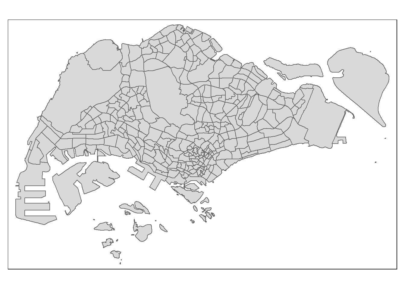

Note

• The source data is in wgs84 coordinates system, hence st_tranform() of sf package is used to theo output sf data.frame into svy21 project coordinates system.

3 Visualiing the Imported Data

We then use the following code chunk to visualise the rainfall stations, the amount of rainfall and the planning subzone boundary.

tmap_options(check.and.fix = TRUE)
tmap_mode("view")

tm_shape(mpsz2019) + #plot boundary map first
  tm_borders() + #Note: if we use tm_polygons, the entire polygon would be shaded, covering the background plot. 
  tm_shape(rfdata_sf) + #plot rainfall stations
  tm_dots(col = "MONTHSUM") #colour the rainfall stations (i.e. the dots) based on the monthly rainfall values 

tmap_mode("plot")

Note

• we use tmap_options(check.and.fix = TRUE) so that tmap would ignore any errors in the map. Without this parameter, if there are unclosed polygons in the map, tmap could fail to plot out the map.

4 Spatial Interpolation: gstat method

4.1 Data Preparation

First, we need to create a grid data object using rast() of terra package as shown in the code chunk below.

grid <- terra::rast(mpsz2019,
                    nrows = 690,  #from the difference between xmax and xmin of mpsz2019 
                    ncols = 1075) # from the difference bwtween ymax and ymin of mpsz2019 

Next, a list called xy will be created by using xyFromCell() of terra package.

xy <- terra::xyFromCell(grid, 
                        1:ncell(grid))

Lastly, we will create a data frame called coop with prediction/simulation locations by using the code chunk below.

coop <- st_as_sf(as.data.frame(xy), 
                 coords = c("x", "y"),
                 crs = st_crs(mpsz2019))
coop <- st_filter(coop, mpsz2019)
head(coop)

Simple feature collection with 6 features and 0 fields
Geometry type: POINT
Dimension:     XY
Bounding box:  xmin: 25883.42 ymin: 50231.33 xmax: 26133.32 ymax: 50231.33
Projected CRS: SVY21 / Singapore TM
                   geometry
1 POINT (25883.42 50231.33)
2  POINT (25933.4 50231.33)
3 POINT (25983.38 50231.33)
4 POINT (26033.36 50231.33)
5 POINT (26083.34 50231.33)
6 POINT (26133.32 50231.33)

4.2 Inverse Distance Weighted (IDW) Method

In the IDW interpolation method, the sample points are weighted during interpolation such that the influence of one point relative to another declines with distance from the unknown point you want to create.

Weighting is assigned to sample points through the use of a weighting coefficient that controls how the weighting influence will drop off as the distance from new point increases. The greater the weighting coefficient, the less the effect points will have if they are far from the unknown point during the interpolation process. As the coefficient increases, the value of the unknown point approaches the value of the nearest observational point.

It is important to notice that the IDW interpolation method also has some disadvantages: the quality of the interpolation result can decrease, if the distribution of sample data points is uneven. Furthermore, maximum and minimum values in the interpolated surface can only occur at sample data points. This often results in small peaks and pits around the sample data points.

4.2.1 Building the models

For the next few steps, we will try building different models with nmax =5, 10 and 15 to see the differences.

nmax = 5

res5 <- gstat(formula = MONTHSUM ~ 1, 
             locations = rfdata_sf, 
             nmax = 5,
             set = list(idp = 0))

nmax = 10

res10 <- gstat(formula = MONTHSUM ~ 1, 
             locations = rfdata_sf, 
             nmax = 10,
             set = list(idp = 0))

nmax = 15

res15 <- gstat(formula = MONTHSUM ~ 1, 
             locations = rfdata_sf, 
             nmax = 15,
             set = list(idp = 0))

4.2.2 Doing interpolation

Now that our model is defined, we can use predict() to actually interpolate, i.e., to calculate predicted values. The predict function accepts:

• A raster—stars object, such as dem
• A model—gstat object, such as g.

The raster serves for two purposes: - Specifying the locations where we want to make predictions (in all methods), and - Specifying covariate values (in Universal Kriging only).

nmax = 5

resp <- predict(res5, coop)

[inverse distance weighted interpolation]

resp$x <- st_coordinates(resp)[,1]
resp$y <- st_coordinates(resp)[,2]
resp$pred <- resp$var1.pred

pred5 <- terra::rasterize(resp, grid, 
                         field = "pred", 
                         fun = "mean")

tmap_options(check.and.fix = TRUE)
tmap_mode("plot")
tm_shape(pred5) + 
  tm_raster(alpha = 0.6, 
            palette = "viridis")

nmax = 10

resp <- predict(res10, coop)

[inverse distance weighted interpolation]

resp$x <- st_coordinates(resp)[,1]
resp$y <- st_coordinates(resp)[,2]
resp$pred <- resp$var1.pred

pred10 <- terra::rasterize(resp, grid, 
                         field = "pred", 
                         fun = "mean")

tmap_options(check.and.fix = TRUE)
tmap_mode("plot")
tm_shape(pred10) + 
  tm_raster(alpha = 0.6, 
            palette = "viridis")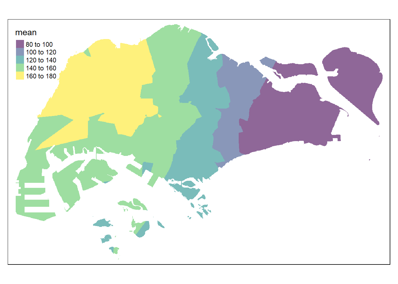

nmax = 15

resp <- predict(res15, coop)

[inverse distance weighted interpolation]

resp$x <- st_coordinates(resp)[,1]
resp$y <- st_coordinates(resp)[,2]
resp$pred <- resp$var1.pred

pred15 <- terra::rasterize(resp, grid, 
                         field = "pred", 
                         fun = "mean")

tmap_options(check.and.fix = TRUE)
tmap_mode("plot")
tm_shape(pred15) + 
  tm_raster(alpha = 0.6, 
            palette = "viridis")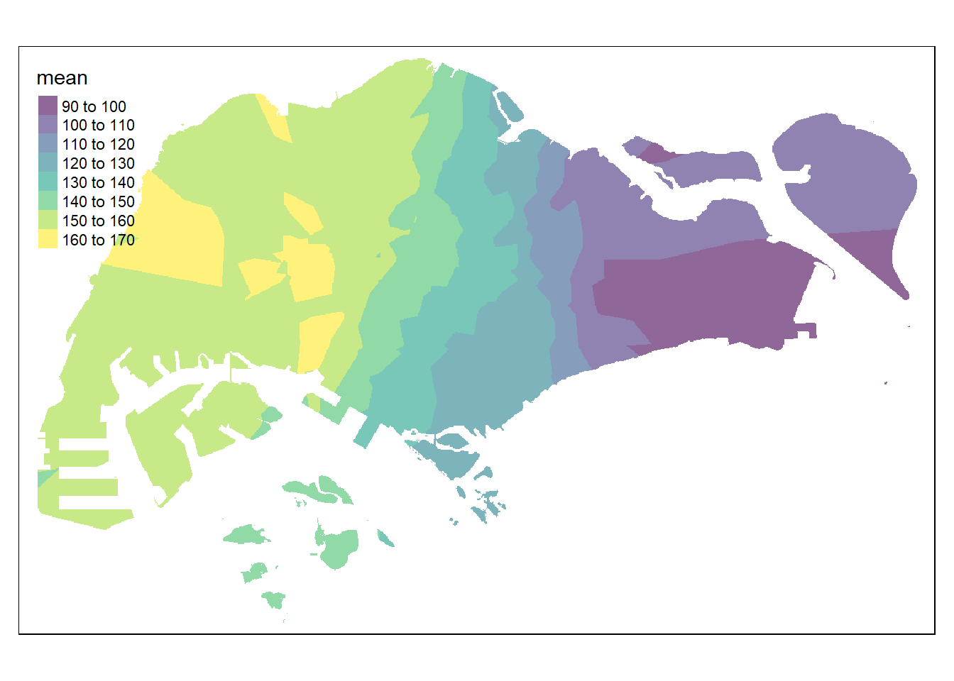

4.3 Kriging Method

Kriging is one of several methods that uses a limited set of sampled data points to estimate the value of a variable over a continuous spatial field. It differs from Inverse Distance Weighted Interpolation in that it uses the spatial correlation between sampled points to interpolate the values in the spatial field: the interpolation is based on the spatial arrangement of the empirical observations, rather than on a presumed model of spatial distribution. Kriging also generates estimates of the uncertainty surrounding each interpolated value.

First, we will calculate and examine the empirical variogram using variogram() of gstat package. The function requires two arguments:

• formula, the dependent variable and the covariates (same as in gstat)
• data, a point layer with the dependent variable and covariates as attributes.

v <- variogram(MONTHSUM ~ 1, 
               data = rfdata_sf)
plot(v)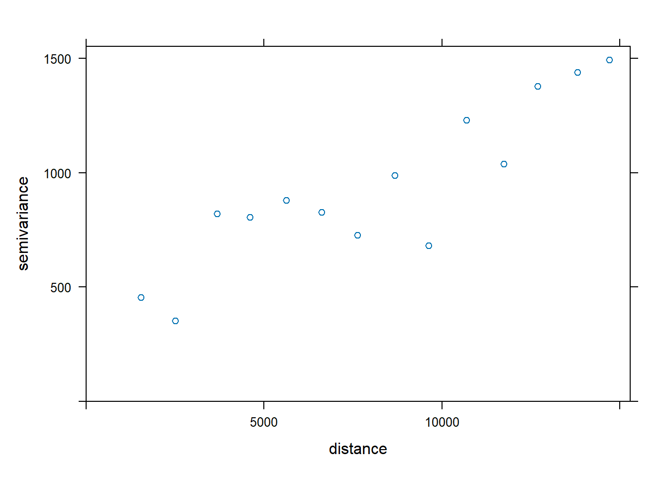

We can then fit an empirical variogram model using fit.variogram().

fv <- fit.variogram(object = v,
                    model = vgm(
                      psill = 0.5, 
                      model = "Sph",
                      range = 5000, 
                      nugget = 0.1))
fv

  model     psill    range
1   Nug 0.1129190    0.000
2   Sph 0.5292397 5213.396

We now visualise how well the observed data fit the model by plotting fv using the following code chunk.

plot(v, fv)

The plot above reveals that the empirical model fits rather well. In view of this, we will go ahead to perform spatial interpolation by using the newly derived model as shown in the code chunk below.

k <- gstat(formula = MONTHSUM ~ 1, 
           data = rfdata_sf, 
           model = fv)
k

data:
var1 : formula = MONTHSUM`~`1 ; data dim = 43 x 2
variograms:
        model     psill    range
var1[1]   Nug 0.1129190    0.000
var1[2]   Sph 0.5292397 5213.396

Now we can use predict() of gstat package to estimate the unknown grids using the following code chunk.

resp <- predict(k, coop)

[using ordinary kriging]

resp$x <- st_coordinates(resp)[,1]
resp$y <- st_coordinates(resp)[,2]
resp$pred <- resp$var1.pred
resp$pred <- resp$pred
resp

Simple feature collection with 314019 features and 5 fields
Geometry type: POINT
Dimension:     XY
Bounding box:  xmin: 2692.528 ymin: 15773.73 xmax: 56371.45 ymax: 50231.33
Projected CRS: SVY21 / Singapore TM
First 10 features:
   var1.pred  var1.var                  geometry        x        y     pred
1   131.0667 0.6608399 POINT (25883.42 50231.33) 25883.42 50231.33 131.0667
2   130.9986 0.6610337  POINT (25933.4 50231.33) 25933.40 50231.33 130.9986
3   130.9330 0.6612129 POINT (25983.38 50231.33) 25983.38 50231.33 130.9330
4   130.8698 0.6613782 POINT (26033.36 50231.33) 26033.36 50231.33 130.8698
5   130.8092 0.6615303 POINT (26083.34 50231.33) 26083.34 50231.33 130.8092
6   130.7514 0.6616697 POINT (26133.32 50231.33) 26133.32 50231.33 130.7514
7   130.6965 0.6617971  POINT (26183.3 50231.33) 26183.30 50231.33 130.6965
8   130.6446 0.6619131 POINT (26233.28 50231.33) 26233.28 50231.33 130.6446
9   130.5958 0.6620184 POINT (26283.26 50231.33) 26283.26 50231.33 130.5958
10  132.5484 0.6542154 POINT (25033.76 50181.32) 25033.76 50181.32 132.5484

In order to create a raster surface data object, rasterize() of terra is used as shown in the code chunk below.

kpred <- terra::rasterize(resp, grid, 
                         field = "pred")
kpred

class       : SpatRaster 
dimensions  : 690, 1075, 1  (nrow, ncol, nlyr)
resolution  : 49.98037, 50.01103  (x, y)
extent      : 2667.538, 56396.44, 15748.72, 50256.33  (xmin, xmax, ymin, ymax)
coord. ref. : SVY21 / Singapore TM (EPSG:3414) 
source(s)   : memory
name        :      last 
min value   :  72.77826 
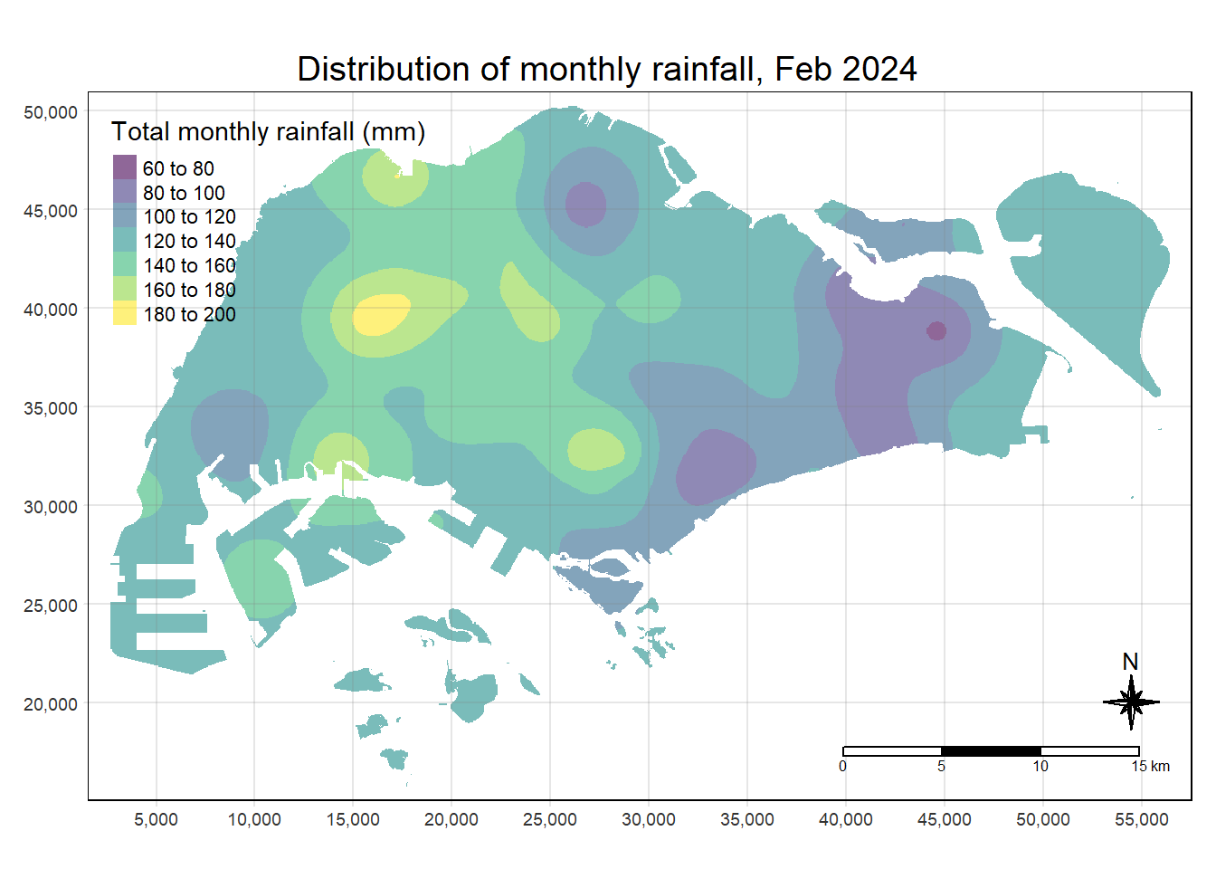
max value   : 195.53284 

Lastly, we will map the interpolated rainfall raster (i.e. kpred) by using tmap.

tmap_options(check.and.fix = TRUE)
tmap_mode("plot")
tm_shape(kpred) + 
  tm_raster(alpha = 0.6, 
            palette = "viridis",
            title = "Total monthly rainfall (mm)") +
  tm_layout(main.title = "Distribution of monthly rainfall, Feb 2024",
            main.title.position = "center",
            main.title.size = 1.2,
            legend.height = 0.45, 
            legend.width = 0.35,
            frame = TRUE) +
  tm_compass(type="8star", size = 2) +
  tm_scale_bar() +
  tm_grid(alpha =0.2)